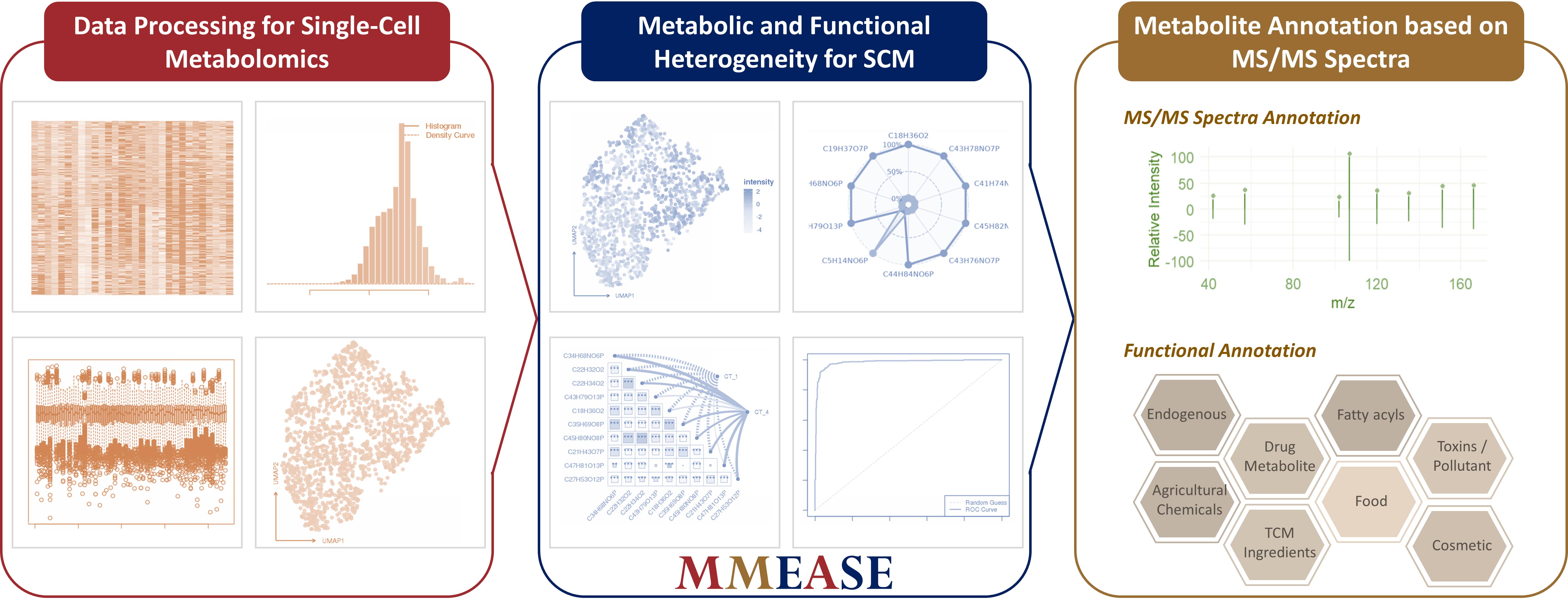
Metabolomics, as the youngest of the omics, provides the readout closest to the phenotype and gives the best view of what chemical processes are taking place in cells (Nat Methods. 18: 1452-6, 2021). Now, metabolomics is shifting to the single-cell level (Nat Biotechnol. 42: 159-62, 2024). Moreover, single-cell metabolomics has regarded as one of seven technologies to watch in 2023 (Nature. 613: 794-7, 2023). A complete analysis procedure of single-cell metabolomics consists of data processing (data filtering, imputation, data transformation, normalization, batch effect removal, etc.), cellular heterogeneity analysis (dimensionality reduction, differential analysis, correlation analysis, classification model construction etc.), metabolite annotation and biological interpretation (Nat Methods. 18: 799-805, 2021). Therefore, it is highly necessary to develop a unified and standardized tool to provide the whole process and enough methods for analyzing single-cell metabolomic data.
MMEASE 2.0 is updated to provide entire analytical workflow of single-cell metabolomics from bulk metabolomics. Specifically, MMEASE 2.0 can (a) provide the most comprehensive workflow for enabling data processing, (b) realize systematical analytical functions for both metabolic heterogeneity and functional heterogeneity, and (c) significantly enhance the capability of metabolite annotation using tandem spectra by integrating the well-established MS2 matching similarity method. All in all, MMEASE 2.0 provides a unique online service of whole analytical workflow of single-cell metabolomics.
The Previous Version of MMEASE can be accessed at: https://idrblab.cn/mmease2021/
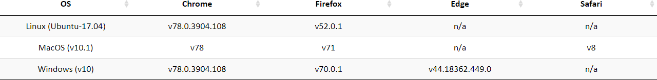
MMEASE 2.0 is powered by R shiny. It is free and open to all users with no login requirement and can be readily accessed by a variety of popular web browsers (such as, Chrome, Firefox, Edge, and Safari) and operating systems (such as, Linux, MacOS, and Windows).
The R Package of MMEASE 2.0 can be accessed at: https://github.com/mmease2025/mmease/
Thanks a million for using and improving MMEASE 2.0, and please feel free to report any errors to Dr. YANG at yangqx@zju.edu.cn.
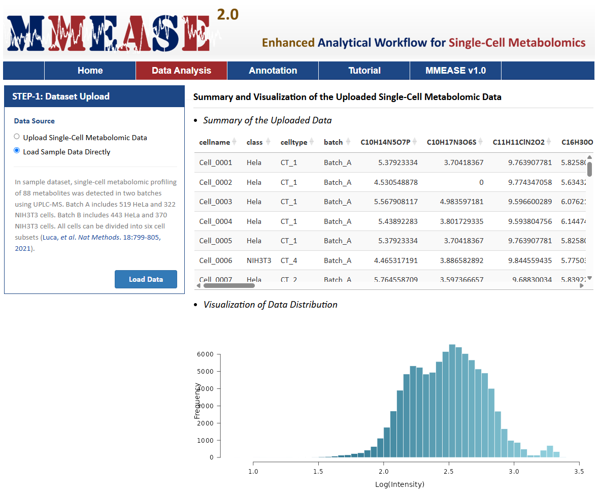
Summary and Visualization of the Uploaded Single-Cell Metabolomic Data
- Summary of the Uploaded Data

- Visualization of Data Distribution
Download the Sample Data of Single-Cell Metabolomics for Testing and File Format Correcting
- Single-Cell Metabolomic Data
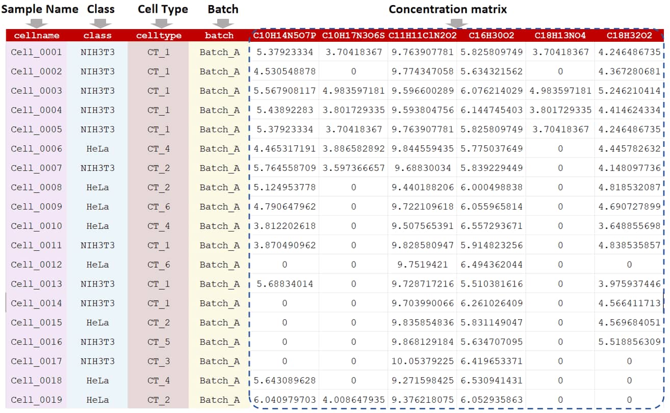
In single-cell metabolomic study, two categories of analysis (metabolic heterogeneity and functional heterogeneity) are popular (Cao et al. Cell Metab. 36: 209-21, 2024; Zhang et al. Nat Commun. 14: 2485, 2023). For metabolic heterogeneity, the variations of metabolic processes across different cell types are studied. For functional heterogeneity, the functional variability of cells particularly in the response to stimuli, biological processes, environmental changes or disease states is performed. As shown in the sample data, cell name, cell classes, cell types, and batch information are required in the first four columns of the input file. In the following columns, the raw peak intensities across all cells are further provided. Unique metabolite IDs or peaks are listed in the first row of the csv file. The sample data of single-cell metabolomic data could be downloaded .
Summary and Visualization of the Uploaded Single-Cell Metabolomic Data
- Summary of the Uploaded Data
- Visualization of Data Distribution
Processing Method of Single-Cell Metabolomics Data
- Data Filtering Method
Single-cell metabolomics is filtered when the tolerable percent of missing values in each metabolite is over the cutoff. The default cutoff is set 0.2 based on "80% rule" (Li et al. Adv Sci. 11: e2305401, 2024).
- Data Imputation Method
KNN (K-nearest neighbor) imputation aims to find k metabolites of interest which are similar to the metabolites with missing value (Liu et al. Anal Chim Acta. 1064: 71-9, 2019).In the KNN algorithm, number of neighbors represents the count of nearest data points, which ranges from 1 to 50, and default value is 10. Max no. of missing data allowed in any row represents the maximum percent of missing data allowed in each row. The minimum is 0, the maximum equals to the number of columns, the default is half of the number of columns. Max no. of missing data allowed in any column indicates the maximum number of missing data permitted in each column, which ranges from 0 to the number of rows, and default value is 80% of the number of rows. The largest block of metabolites imputed refers to the maximum number of metabolite blocks imputed, which ranges from 1 to the number of metabolites.
1/5 of min positive value of corresponding metabolite method aims to handle missing values with a small value derived from the data itself (Li et al. Adv Sci. 11: e2305401, 2024).
- Data Transformation Method
G-log transformation applies a generalized logarithm function that incorporates a small constant to handle zero or near-zero values, ensuring numerical stability (Li et al. Adv Sci. 11: e2305401, 2024).
Log 2 transformation applies a base-2 logarithm to each data point and compresses large values while expanding small values (Liu et al. Anal Chem. 95: 7127-33, 2023).
Log 10 transformation applies the base-10 logarithm to reduce the data range and stabilize variance across data with large dynamic ranges (Rappez et al. Nat Methods. 18: 799-805, 2021).
- Data Normalization Method
Auto Scaling is also referred as unit variance scaling to adjust metabolite variances, which achieves efficacy by using the standard deviation as scaling factor to scale all of the metabolites(Li et al. Adv Sci. 11: e2305401, 2024).
Mean Normalization is used to eliminate background effect where the means of the intensities for each cell are forced to be equal to one another (Ejigu et al. OMICS. 17: 473-85, 2013).
Median Normalization normalizes each cell to make the median of the metabolite abundances across samples equal to each other (Wang et al. Anal Chem. 75: 4818-26, 2003).
For MS Total Useful Signal (MSTUS), the intensity of each cell is divided by the sum based on the assumption that there is an equivalence between increased intensities and decreased intensities (Saccenti et al. J Proteome Res. 16: 619-34, 2017).
Single Internal Standard can be applied to normalize data by subtracting metabolite abundance of a single internal standard from the abundances of the metabolites in each cell (De Livera et al. Anal Chem. 84: 10768-76, 2012). To select the column of single IS (internal standard), IS represents the column number as the reference for data normalization. The value ranges from 1 to the number of columns.
- Batch Correction Method
ComBat uses an empirical Bayes framework to adjust for batch effects and removes batch-specific mean and variance while retaining the overall data structure (Rappez et al. Nat Methods. 18: 799-805, 2021).
Limma fits linear models to the expression data for each feature across cells using empirical Bayes to improve variance estimation (Misra et al. Methods Mol Biol. 2064: 191-217, 2020).
Summary and Visualization of Single-Cell Metabolomic Data after Data Processing
- Visualization of Matrix Distribution after Data Imputation
Methods of Data Analysis in Single-Cell Metabolomics
- Metabolic Heterogeneity
For metabolic heterogeneity, the variations of metabolic processes or cell states across different cell types are studied (Cao et al. Cell Metab. 36: 209-221, 2024).
- Functional Heterogeneity
For functional heterogeneity, the functional variability of cells, such as the response to stimuli, biological processes, environmental changes or disease states is explored (Zhang et al. Nat Commun. 14: 2485, 2023).
- Dimensionality Reduction
UMAP visualization is used to visualize high-dimensional data in a lower-dimensional space for complex single-cell metabolomic data by preserving both local and global structures (Qin et al. Nat Commun. 15: 4387, 2024).
t-SNE visualization focuses on preserving local structure by minimizing the divergence between the probability distributions of high- and low-dimensional data points. (Xu et al. Adv Sci. 11: e2306659, 2024).
- Differential Analysis
Fold change (FC) is the ratio of mean levels between two groups for each metabolite in single-cell metabolomics.
One-way ANOVA compares two groups to identify significant differences in single-cell metabolomics.
Orthogonal partial least squares discriminant analysis (OPLS-DA) improves PLS-DA by using a single component as a predictor for group discrimination, with other components orthogonal to it in single-cell metabolomics.
VSRF measures the variable importance of potentially influential parameters through the percent increase of the mean squared error. The strength of VSRF lies in its flexibility and interpretability.
KWT is a non-parametric statistical test, which is applied to test the difference between multiple samples when the underlying population distributions are nonnormal or unknown. A Kruskal-Wallis Test of the feature among various classes reveals a statistically significant difference.
SVM-RFE is an efficient feature selection technique, which can measure the weights of the features according to the support vectors, noise, and non-informative variables in the high dimension data may affect the hyper-plane of the SVM learning model.
In Student`s t-test, the test statistic follows a t-distribution if the null hypothesis holds in single-cell metabolomics.
- Visualization of Specific Differential Metabolite
Relative intensity of differential metabolites refers to the normalized metabolite abundance across all cells in UMAP.
A boxplot shows a box with lines extending from each side, representing the range of a differential metabolite.
- Visualization of Multiple Differential Metabolites
Heatmap of differential metabolites highlights significant differences of multiple Metabolites among different groups.
In a radargram, differential metabolites are plotted along axes radiating from a central point in a circular format.
- Correlation Analysis of Cell Populations
In correlation scatter matrix, each plot represents the correlation between two metabolites to visualize the linear relationships and patterns.
Heatmap of mental test correlation can visualize the correlation between the results of multiple mental tests.
- Select a Classification Method
Adaptive boosting (AdaBoost) can build a much better classifier by boosting the performance of the weak classification algorithm.
In Bagging, a random sample in the training set is selected with replacement and the individual data points can be chosen more than once.
Decision trees (DT) can provide high classification accuracy with a simple representation of gathered knowledge.
For k-nearest neighbor (KNN), the core of this classifier depends mainly on measuring the distance or similarity between the tested and the training examples.
Linear discriminate analysis (LDA) takes the mean value for each class and considers variants in order to make predictions assuming a Gaussian distribution.
Naive Bayes (NB) implements the Bayes theorem for the computation and uses class levels for representing as feature values or vectors of predictors for classification.
Partial least squares (PLS) can form linear combinations of the predictors in a supervised manner, and regresses the response on these latent variables.
Random Forest (RF) builds decision trees from random data samples and makes predictions based on each tree.
Support Vector Machine (SVM) finds a hyperplane in N-dimensional space to distinctly classify data points.
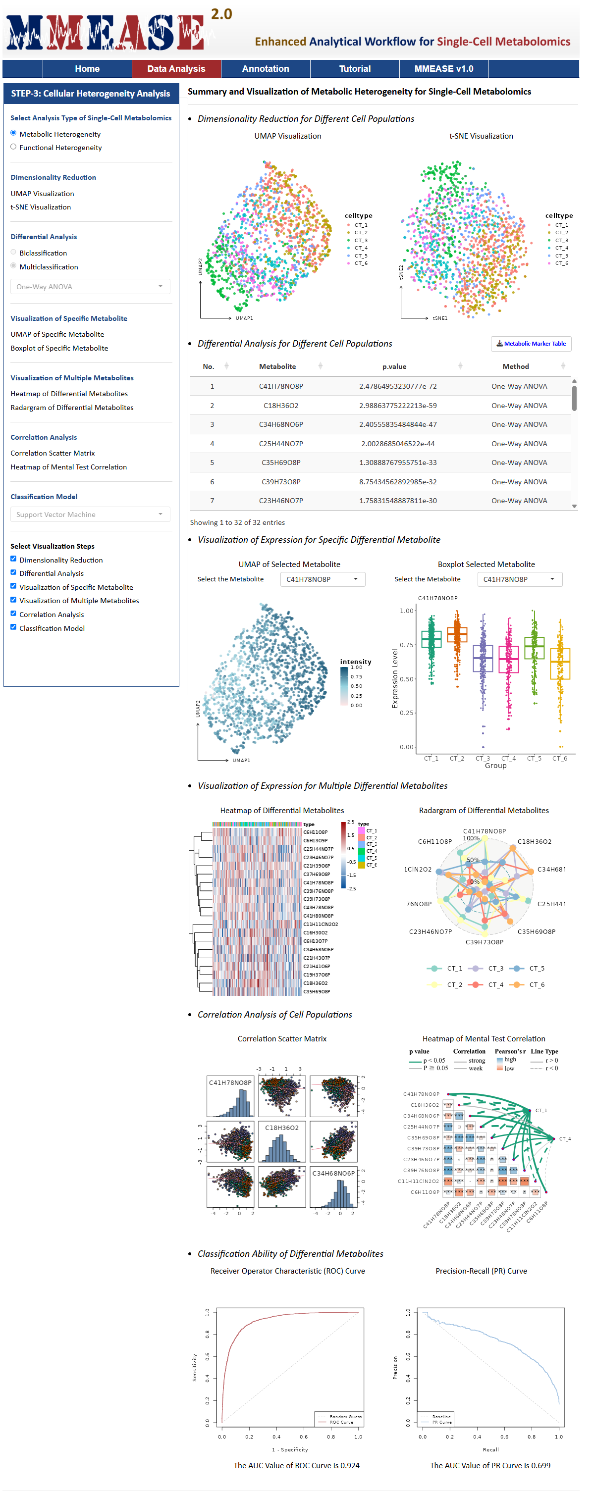
Summary and Visualization of Metabolic Heterogeneity for Single-Cell Metabolomics
- Dimensionality Reduction for Different Cell Populations
UMAP Visualization
t-SNE Visualization
- Visualization of Expression for Specific Differential Metabolite
UMAP of Selected Metabolite
Boxplot Selected Metabolite
Select the Metabolite
Select the Metabolite
Select the Metabolite
Select the Metabolite
- Visualization of Expression for Multiple Differential Metabolites
Heatmap of Differential Metabolites
Radargram of Differential Metabolites
- Correlation Analysis of Cell Populations
Correlation Scatter Matrix
Heatmap of Mental Test Correlation
- Classification Ability of Differential Metabolites
Receiver Operator Characteristic (ROC) Curve
Precision-Recall (PR) Curve
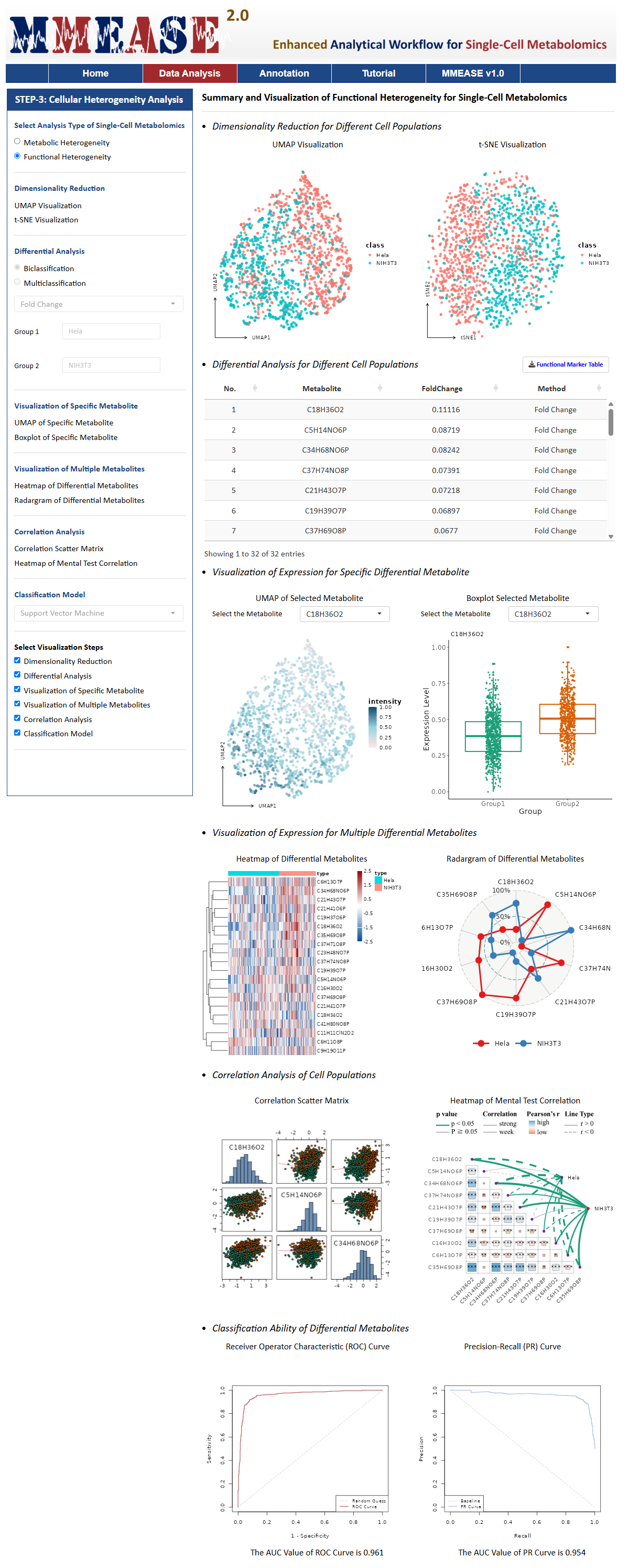
Summary and Visualization of Functional Heterogeneity for Single-Cell Metabolomics
- Dimensionality Reduction for Different Cell Populations
UMAP Visualization
t-SNE Visualization
- Visualization of Expression for Specific Differential Metabolite
UMAP of Selected Metabolite
Boxplot Selected Metabolite
Select the Metabolite
Select the Metabolite
Select the Metabolite
Select the Metabolite
- Visualization of Expression for Multiple Differential Metabolites
Heatmap of Differential Metabolites
Radargram of Differential Metabolites
- Correlation Analysis of Cell Populations
Correlation Scatter Matrix
Heatmap of Mental Test Correlation
- Classification Ability of Differential Metabolites
Receiver Operator Characteristic (ROC) Curve
Precision-Recall (PR) Curve
High Resolution Metabolite Annotation and Cell-based Biological Interpretation
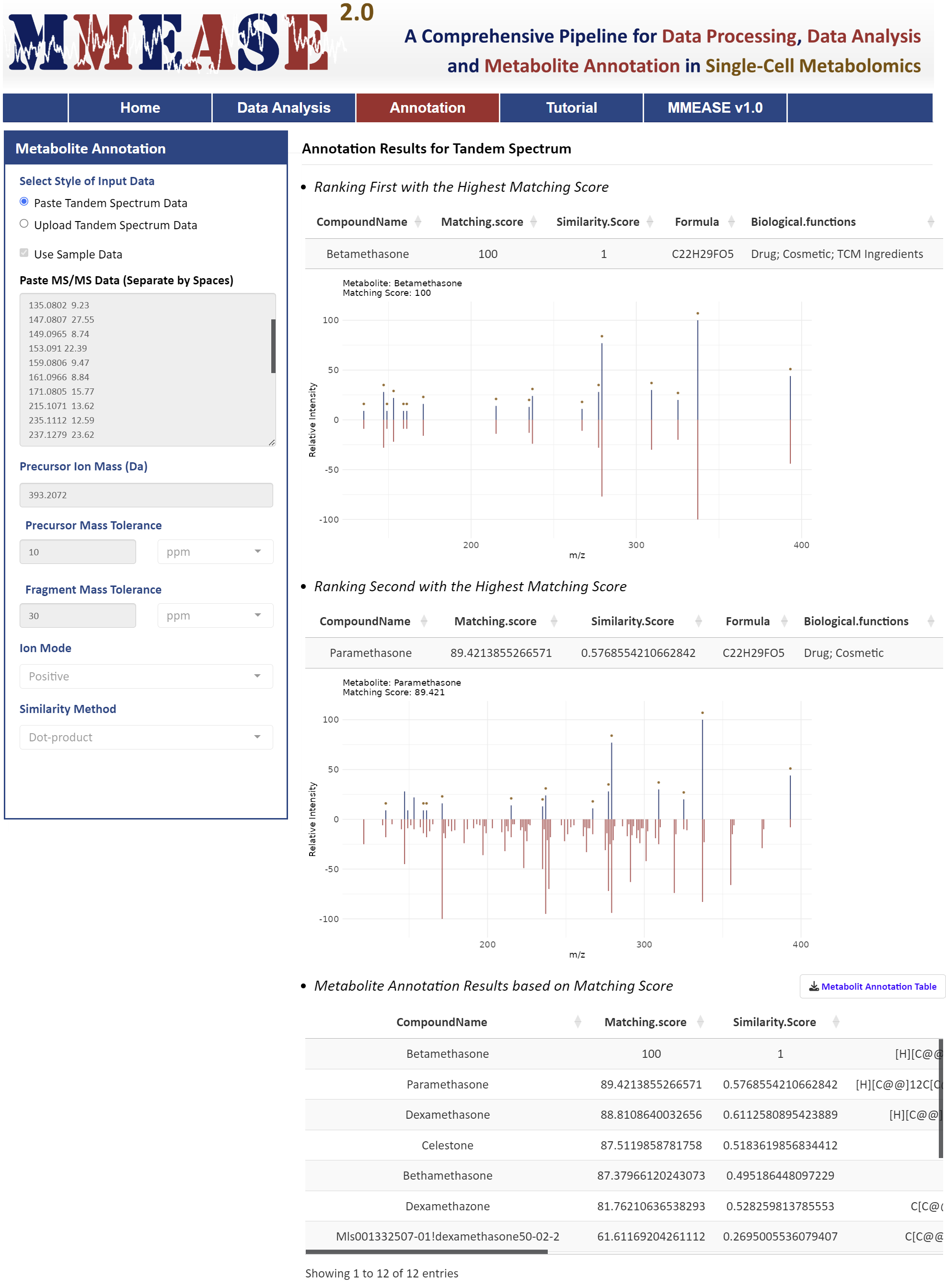
- Metabolite Annotation Using Tandem Spectra
Metabolite annotation for single-cell metabolomics in MMEASE 2.0 is supported by a comprehensive reference spectra database organized into several libraries including biology, lipid, and exposome. These databases are curated from public sources like HMDB, MoNA, LipidBlast, GNPS, and KEGG, with MS2 spectra fragments annotated into formulas using BUDDY (Xing, et al. Nat Methods. 20: 881-90, 2023). Two widely used methods, dot product and spectral entropy, are implemented to evaluate MS2 matching similarity (Pang, et al. Nat Commun. 1:3675, 2024).
- Metabolite Annotation for Biological Functions
Metabolites are classified into differential biological or functional groups through literature reviews and information from public sources such as HMDB, T3DB, KEGG, and DrugBank, providing insights into exogenous factors like food, drugs, toxins, and pollutants (Yang, et al. J Proteomics. 232:104023, 2021). In the paste box, two columns separate by spaces are needed. In the uploaded CSV file, two columns separate by commas are needed. The m/z values of the MS2 spectra are in the first column and the relative abundances of the responding m/z values are in the second column. The sample data of tandem spectrum could be downloaded .
Annotation Results for Tandem Spectrum
- Ranking First with the Highest Matching Score
- Ranking Second with the Highest Matching Score
- Ranking Third with the Highest Matching Score
- Metabolite Annotation Results based on Matching Score
Table of Contents
1. The Compatibility of Browser and Operating System (OS)
2. Required Formats of the Input Files
3. Step-by-step Instruction on the Usage of MMEASE 2.0
3.1 Uploading the Customized Single-Cell Metabolomic Data or the Sample Data Provided in MMEASE 2.0
3.2 Data Processing for Single-Cell Metabolomics
3.3 Data Analysis for Single-Cell Metabolomics
3.4 Metabolite Annotation for Single-Cell Metabolomics
MMEASE 2.0 is powered by R shiny. It is free and open to all users with no login requirement and can be readily accessed by a variety of popular web browsers and operating systems as shown below.
In general, the file required at the Step 1 of MMEASE 2.0 should be a sample-by-feature matrix in a csv format. In the uploaded dataset, the first 4 columns of the input file contain cell name, class, cell type, and batch, and are kept as "Cell Name","Class", "Cell Type" and "Batch". In the following columns of the input file, metabolites’ raw intensities across all samples are further provided. Chemical formulas of each metabolite are listed in the first row of the csv file. The sample data of single-cell metabolomic data could be downloaded .
This website is free and open to all users and there is no login requirement, and can be readily accessed by all popular web browsers including Google Chrome, Mozilla Firefox, Safari and Internet Explorer 10 (or later), and so on. Analysis is started by clicking on the "Analysis" panel on the homepage of MMEASE 2.0. The collection of web services and the whole process provided by MMEASE 2.0 can be summarized into 4 steps: (3.1) Upload Single-Cell Metabolomic Data, (3.2) Data Processing for Single-Cell Metabolomics, (3.3) Data Analysis for Single-Cell Metabolomics, and (3.4) Metabolite Annotation for Single-Cell Metabolomics.

There is one radio checkboxes in STEP-1 on the left side of the Analysis page. Users can choose to upload their own single-cell metabolomics data or to directly load sample data. After selecting the corresponding radio checkboxes, datasets provided by the users for further analysis can be then directly uploaded by clicking "Browse". Preview of the uploaded data is subsequently provided on the web page.
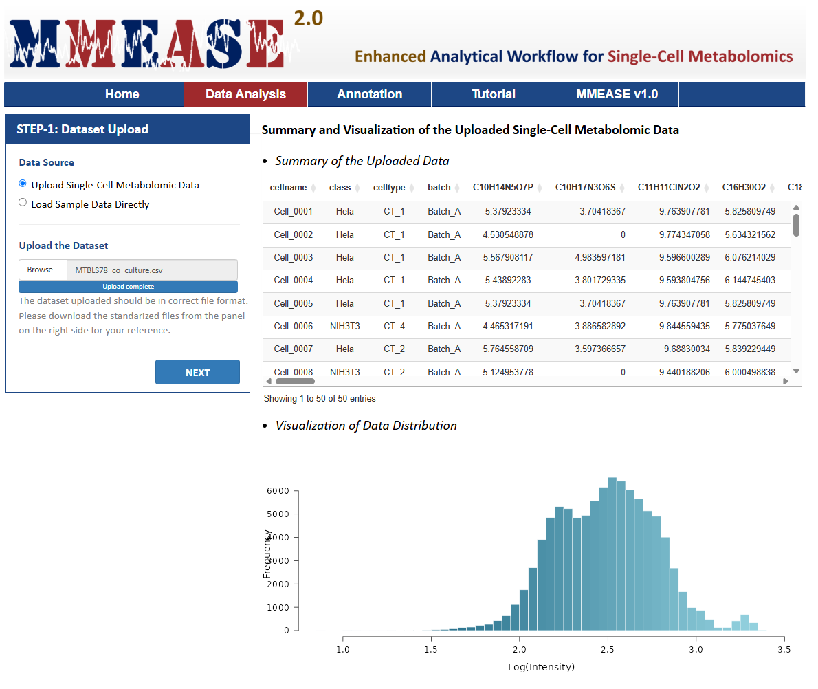
The sample data are also provided in this step facilitating a direct access of MMEASE 2.0. In this sample dataset, the single-cell metabolomic data collected from 962 HeLa and 692 NIH3T3 cells were selected as the example dataset (Luca Rappez, et al. Nat Methods. 18:799-805,2021). By clicking the Load Data button, the sample dataset selected by the users can be uploaded for further analysis.
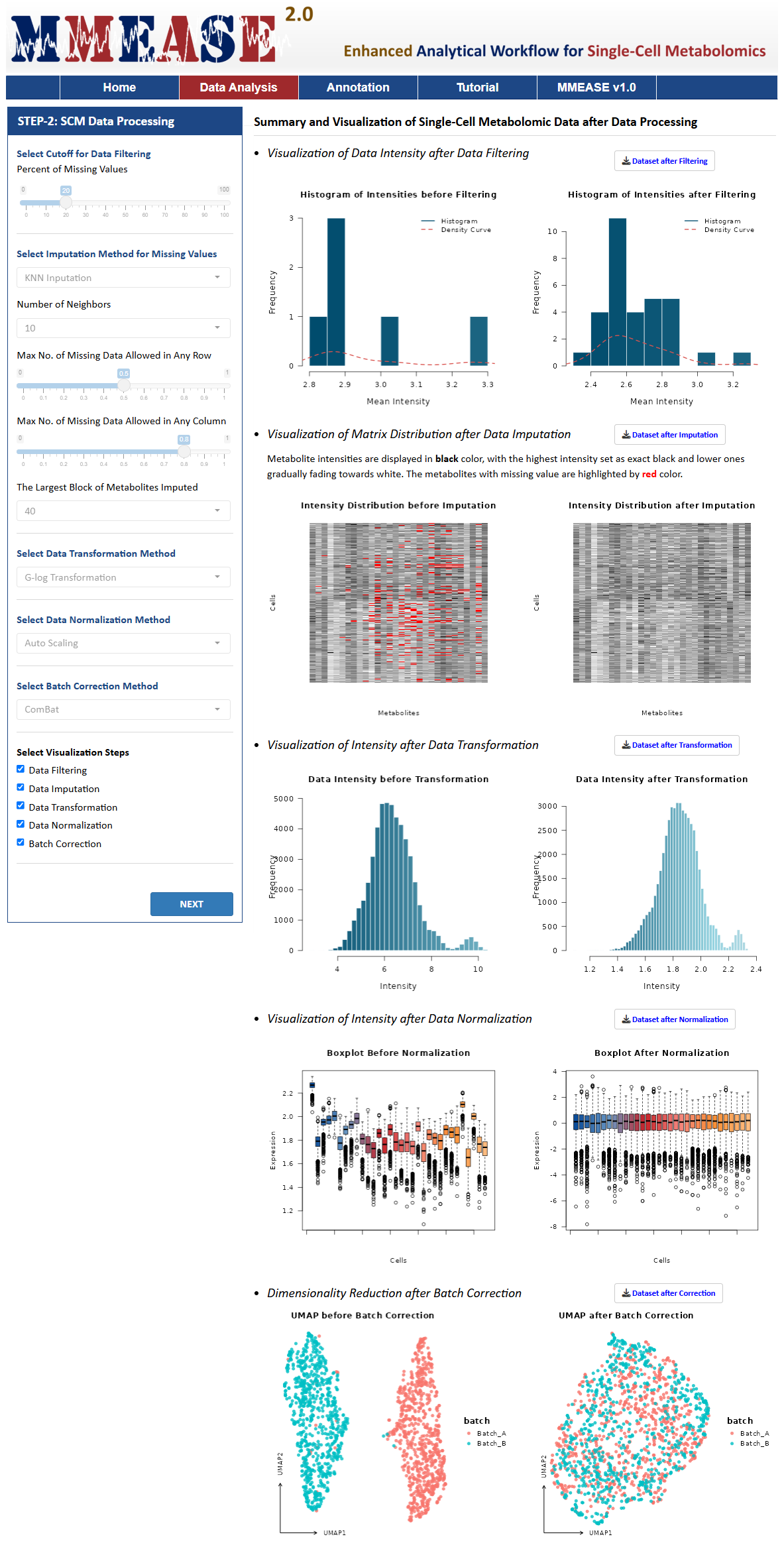
MMEASE 2.0 provides data processing including Data Filtering, Data Imputation, Data Transformation, Data Normalization, and Batch Correction. Single-cell metabolomic data is filtered when the tolerable percent of missing values in each metabolite is over the set cutoff. The cutoff of the tolerable percent of missing values could be set by users and default value is 0.2 based on "80% rule" in metabolomics (Chen, et al. Anal Chem. 89:5342-8, 2017). A detailed explanation of the methods used in each process is provided in this Manual. After selecting or defining preferred methods or parameters, please proceed by clicking the "PROCESS" button, the summary and visualization of single-cell metabolomic data are automatically generated. All resulting data and figures can be downloaded by clicking the corresponding "Download" button.
Data Filtering
After data filtering, proper handling of missing values is that the shapes of the histogram and density curve become more regular. The processed histogram exhibits a more reasonable range on the x-axis, a frequency distribution on the y-axis that aligns better with expectations, and no noticeable abnormal troughs or empty intervals.
Data Imputation
After data imputation, good performance exhibits that there a significant reduction in blank areas representing missing values, a more complete data matrix, and a data distribution morphology that remains largely consistent before and after imputation.
Data Imputation Method
a. KNN Inputation
KNN imputation (K-nearest Neighbor Imputation) method aims to find k metabolites of interest which are similar to the metabolites with missing value. The similarity is measured by Euclidean distance and the missing value is imputed by the weighted average of those k metabolites (Tang,et al. J Brief Bioinform. 2:621-636 ,2020).In the KNN algorithm, number of neighbors represents the count of nearest data points, which ranges from 1 to 50, and default value is 10. Max no. of missing data allowed in any row represents the maximum percent of missing data allowed in each row. The minimum is 0, the maximum equals to the number of columns, the default is half of the number of columns. Max no. of missing data allowed in any column indicates the maximum number of missing data permitted in each column, which ranges from 0 to the number of rows, and default value is 80% of the number of rows. The largest block of metabolites imputed refers to the maximum number of metabolite blocks imputed, which ranges from 1 to the number of metabolites.
b. 1/5 of Minimum Positive Value
1/5 of Minimum Positive Value of corresponding variables imputation strategy aims to handle missing or zero values with a small value derived from the data itself (1/5 of the smallest positive value of the same variable). (Li, et al. Adv Sci. 9:e2305401, 2024).
Data Transformation
After data transformation, optimal performance demonstrates that histogram more closely resembles a unimodal and roughly symmetric bell-shaped curve of a normal distribution, which exhibits a narrower width and mitigating the influence of outliers represented by isolated bars in the original histogram.
Data Transformation Methods
a. G-log Transformation
G-log transformation applies a generalized logarithm function that incorporates a small constant to handle zero or near-zero values, ensuring numerical stability. By compressing large values and expanding smaller ones, it balances the data scale while preserving the relative differences between variables (Li, et al. Adv Sci. 9:e2305401, 2024).
b. Log2 Transformation
Log2 transformation aims to make the distribution of data more symmetric and closer to normal, which is beneficial for statistical analysis. It applies a base-2 logarithm to each data point and compresses large values while expanding small values, creating a balanced scale (Liu, et al. Anal Chem. 18:7127-7133, 2023).
c. Log10 Transformation
Log10 transformation applies the base-10 logarithm to each data point. It compresses large values and stretches small values to reduce the data range and stabilize variance across datasets with large dynamic ranges (Luca Rappez, et al. Nat Methods. 18:799-805, 2021).
Data Normalization
After data normalization, superior performance exhibits that medians across boxplots converge toward a similar level, box lengths become more consistent, effectively controlling data dispersion and variability between different groups, and outliers are significantly reduced and distributed more uniformly.
Data Normalization Methods
a. Auto Scaling
Auto Scaling is also referred as unit variance scaling, which is a metabolite-based normalization method to adjust metabolite variances. AUT achieves its efficacy by using the standard deviation as scaling factor to scale all of the metabolic signals (Kohl SM, et al. Metabolomics. 8:146-60, 2012).
b. Mean Normalization
Mean Normalization is a sample-based normalization method that eliminates background effects by equalizing the means of intensities across samples, making them comparable (Ejigu BA, et al. OMICS. 17:473-85, 2013;Andjelkovic V, et al. Plant Cell Rep. 25:71-9, 2006).
c. Median Normalization
Median Normalization is one of the commonly used sample-based normalization methods which do not take any internal standards, normalizing each sample to make the median of the metabolite abundances across samples equal to each other (Wang W, et al. Anal Chem. 75:4818-26, 2003).
d. MS Total Useful Signal (MSTUS)
MS Total Useful Signal (MSTUS), also referred as MS total useful signal, is a sample-based normalization method where the intensity of each spectrum is divided by the sum of intensities of all spectra based on the assumption that there is an equivalence between increased intensities and decreased intensities (Saccenti E, et al. J Proteome Res. 16:619-34, 2017;Warrack BM, et al. J Chromatogr B. 877:547-52, 2009).
e. Single Internal Standard Normalization
Single Internal Standard (SIS) normalizes data by subtracting the log abundance of a single internal standard from the log abundances of metabolites in each sample (De Livera AM, et al. Anal Chem. 84:10768-76, 2012;Jonas Gullberg, et al. Anal biochem. 2:283-95, 2004). It assumes that all metabolites experience the same amount of unwanted variation, which can be measured by the internal standard (De Livera AM, et al. Anal Chem. 84:10768-76, 2012).To select the column of single IS (internal standard), IS represents the column number as the reference for data normalization. The value ranges from 1 to the number of columns.
Batch Correction
A successful batch correction should result in data points from different batches being better mixed and no longer distinctly separated in the UMAP plot, which produces a cleaner plot without obvious isolated points, with a more regular distribution of post-correction data points and reduced noise.
Batch Correction Methods
a. ComBat
ComBat is a standard choice for batch correction in omics data analysis. It uses an empirical Bayes framework to adjust for batch effects and removes batch-specific mean and variance while retaining the overall data structure (Luca Rappez,et al. Nat Methods. 18:799-805, 2021;Liu, et al. Anal Chem. 18:7127-7133, 2023). The method can accommodate known covariates (e.g., experimental groups) to prevent overcorrection of biological differences.
b. Limma
Limma is a statistical software package designed for analyzing gene expression data with complex experimental designs and batch effects. Limma fits linear models to the expression data for each gene across samples. It uses empirical Bayes methods to improve variance estimation, particularly for small sample sizes (Biswapriya B Misra, et al. Methods Mol Biol. 2064:191-217, 2020).
Metabolic Heterogeneity
Metabolic Heterogeneity is the variation analysis of metabolic processes and profiles across different cell types, such as T cell and B cell. For this analysis type, MMEASE 2.0 provides the following six analysis processes, Dimensionality Reduction, Differential Analysis, Visualization of Specific Metabolite, Visualization of Multiple Metabolites, Correlation Analysis, and Classification Model.
Functional Heterogeneity
Functional Heterogeneity is the variability analysis of the functional characteristics of cells, particularly in their response to stimuli, biological processes, or environmental changes. For example, cells of the same type exhibit significant differences in metabolites between normal and cancerous tissues. For this analysis type, MMEASE 2.0 also provides the following six analysis processes, Dimensionality Reduction, Differential Analysis, Visualization of Specific Metabolite, Visualization of Multiple Metabolites, Correlation Analysis, and Classification Model.
A detailed explanation of the methods used in each process is provided in this Manual. After selecting or defining preferred methods or parameters, please proceed by clicking the "PROCESS" button, the summary and visualization of single-cell metabolomic data are automatically generated. All resulting data and figures can be downloaded by clicking the corresponding "Download" button.
Dimensionality Reduction
UMAP Visualizations
UMAP is a dimensionality reduction technique used for visualizing high-dimensional data in a lower-dimensional space. It is particularly useful for visualizing complex datasets, such as single-cell metabolomic data, by preserving both local and global structures in the data.
t-SNE Visualizations
t-SNE is used for visualizing high-dimensional data in lower-dimensional spaces, typically 2D or 3D. It focuses on preserving the local structure of the data by minimizing the divergence between probability distributions of high-dimensional and low-dimensional data points.
Differential Analysis
Fold Change
Fold change (FC) is the ratio of mean abundance values between two groups for each metabolite in single-cell metabolomics. FC is to compare the absolute value change between means of two groups. A threshold needs to be defined, if fold change value exceeds this threshold, the metabolite will be reported as significant(Bertini I, et al. Cancer Res. 72(1):356-64, 2012).For fold change, log2FC was utilized to identify the differential metabolites.
One-Way ANOVA
One-Way ANOVA is a commonly used statistical method that compares the means of two or more independent groups to determine if their population means are significantly different (Wu, et al. Biochem Biophys Res Commun. 358:1108-13, 2007).For one-way ANOVA, p value was utilized to identify the differential metabolites.
Orthogonal Partial Least Squares Discriminant Analysis (OPLS-DA)
OPLS-DA improves PLS-DA by using a single component as a predictor for group discrimination, with other components orthogonal to it. It has been widely applied in metabolomics to identify biomarkers in amyotrophic lateral sclerosis and detect diagnostic markers for early-stage ovarian cancer (H Blasco, et al. Eur J Neurol. 2:346-53, 2015).For OPLS-DA, VIP was utilized to identify the differential metabolites.
Partial Least Squares-Discriminant Analysis (PLS-DA)
In metabolomic study, partial least squares-discriminant analysis (PLS-DA) is the most well-known tool to perform classification and regression. One of the perceived advantages of PLS-DA is that it can analyze highly collinear and noisy data (Gromski PS, et al. Anal Chim Acta. 879:10-23, 2015).For PLS-DA, VIP was utilized to identify the differential metabolites.
Variable Selection from Random Forests (VSRF)
VSRF is a recursive feature elimination method that starts with all features and iteratively removes the least important one, based on random forest importance scores, until no features remain. The features are then ranked by the deletion sequence, with the top-ranked feature being the last deleted. RF-RFE has been used to study fatty acid metabolism deregulation in liver diseases (Zhou, et al. Anal Bioanal Chem. 1:203-13, 2012).For VSRF, importance rating of variables was utilized to identify the differential metabolites.
Student’ t-Test
Student’ t-Test is a statistical hypothesis test in which the test statistic follows a Student’ s t-distribution if the null hypothesis is supported. Student’ t-Test has been widely applied in metabolomics analysis to predict early-onset preeclampsia (Ray O Bahado-Singh, et al. Am J Obstet Gynecol. 4:530.e1-530.e10, 2015), and determinate the untargeted metabolomic profile (Arnald Alonso, et al. Front Bioeng Biotechnol. 5:3:23, 2015).For student’ t-test, p value was utilized to identify the differential metabolites.
Kruskal–Wallis Test (KWT)
Kruskal-Wallis Test (KWT) is a non-parametric statistical test and is applied when the goal is to test the difference between multiple samples and the underlying population distributions are nonnormal or unknown (Abenavoli, et al. J Am Osteopath Assoc. 120: 647-54, 2020). A Kruskal-Wallis Test of the feature among various classes reveals a statistically significant difference. In metabolomics studies, Kruskal-Wallis Test is widely applied to identify metabolomic markers (Sawicka-Smiarowska E, et al. J Clin Med. 10: 5074, 2021).For KWT, p value was utilized to identify the differential metabolites.
Support Vector Machine-Recursive Feature Elimination (SVM-RFE)
Support vector machine-recursive feature elimination (SVM-RFE) is an efficient feature selection technique and has shown promising applications in the analysis of the metabolome data. SVM-RFE measures the weights of the features according to the support vectors, noise and non-informative variables in the high dimension data may affect the hyper-plane of the SVM learning model (Lin X, et al. J Chromatogr B. 910: 149-55, 2012). Nowadays, SVM-RFE is widely used in metabolomics studies for revealing metabolite biomarkers (Gromski PS, et al. Anal Chim Acta. 829: 1-8, 2014).For SVM-RFE, in recursive feature elimination, the features corresponding to the highest accuracy are identified as the differential metabolites.
Visualization of Specific Metabolite
UMAP of Specific Metabolite
UMAP of Specific Metabolite refers to a two-dimensional visualization technique using the Uniform Manifold Approximation and Projection (UMAP) algorithm to display the distribution and clustering of specific metabolite across samples or conditions. This approach helps to identify patterns, relationships, and variations in the levels of selected metabolites within complex datasets, providing insights into their roles and significance in biological processes.
Boxlplot of Specific Metabolite
A boxplot of specific metabolite is a graphical representation used to display the distribution of metabolite levels across different groups or conditions. It summarizes the data by showing the median, interquartile range (IQR), and potential outliers, allowing for the comparison of metabolite abundances and the identification of variations or significant differences between groups.
Visualization of Multiple Metabolites
Heatmap of Differential Metabolites
A Heatmap of Differential Metabolites is a graphical representation that displays the intensity of metabolic changes between different conditions or groups, using colors to indicate the levels of metabolites across samples, often highlighting significant differences.
Radar Map of Differential Metabolites
Radar Map is a graphical representation used to display multivariate data, where multiple variables are plotted along axes that radiate from a central point, allowing for a visual comparison of different categories or conditions in a circular format.
Correlation Analysis
Correlation Scatter Matrix
Correlation Scatter Matrix is a grid of scatter plots that shows the relationships between multiple variables. Each plot represents the correlation between two variables, allowing for the visualization of linear relationships and patterns in the data.
Heatmap of Mental Test Correlation
Heatmap of Mental Test Correlation is a graphical representation that visualizes the correlation between the results of multiple mental tests. It uses color gradients to indicate the strength and direction of the relationships, with higher correlations shown in darker or more intense colors.
Classification Model
Adaptive Boosting (AdaBoost)
The idea of boosting is to take a weak classifier, and use it to build a much better classifier, thereby boosting the performance of the weak classification algorithm. The most popular boosting algorithm is AdaBoost because it is adaptive (Dou L, et al. J Proteome Res. 20:191-201, 2021).For AdaBoost method, the parameters are set as default.
Bagging
In bagging, a random sample in the training set is selected with replacement and the individual data points can be chosen more than once. After several data samples are generated, these weak models are then trained independently, and the average of the predictions yield a more accurate estimate (Datta S, et al. BMC Bioinformatics. 11:427, 2010).For bagging method, the parameters are set as default.
Decision Trees (DT)
Decision tree is a reliable and effective decision making technique that provide high classification accuracy with a simple representation of gathered knowledge (Luna JM, et al. Proc Natl Acad Sci U S A. 116:19887-93, 2019). The most commonly used applications of decision trees are data mining and data classification in different areas of medical decision making (Podgorelec V, et al. J Med Syst. 26:445-63, 2002).For decision tree, the number of boosting iterations is set as 10, and other parameters is set as default.
K-Nearest Neighbor (KNN)
KNN is a non-parametric algorithm without any assumption on underlying data (Wang, et al. IEEE Trans Neural Netw Learn Syst. 31:1544-56, 2020). KNN is one of the simplest and most common classifiers and the core of this classifier depends mainly on measuring the distance or similarity between the tested examples and the training examples (Abu Alfeilat HA, et al. Big Data. 7:221-48, 2019. 26:445-63, 2002).For KNN, Minkowski distance is set 1, the kernel is set "triangular", and the parameters are set as default.
Linear Discriminat Analysis (LDA)
LDA is a widely used classification method with ready implementability and close relationships with many modern machine learning techniques (Ye, et al. Neural Netw. 105:393-404, 2018). Now, LDA helps to represent data for more than two classes. Linear discriminant analysis takes the mean value for each class and considers variants in order to make predictions assuming a Gaussian distribution.For LDA, the parameters are set as default.
Naive Bayes (NB)
The Naive Bayes implements the Bayes theorem for the computation and uses class levels for representing as feature values or vectors of predictors for classification (Miasnikof P, et al. BMC Med. 13:286, 2015). Naive Bayes classifiers have high accuracy and speed on large datasets (Zhang, et al. Food Chem Toxicol. 143:111513, 2020).For NB, Laplace is set as 3, indicating positive double controlling Laplace smoothing. The parameters are set as default.
Random Forest (RF)
The random forest classifier consists of multiple decision trees just as a forest has many trees. It makes decision trees based on a random selection of data samples and get predictions from every tree (de Santana FB, et al. Food Chem. 293:323-32, 2019). The random forest classification offers a rapid, sensitive, and accurate solution for identifying signatures in omics data (Roguet A, et al. Microbiome. 6:185, 2018).For RF, importance is set TRUE, indicating importance of predictors are assessed, proximity is set TRUE, indicating proximity measure among the rows is calculated, and the parameters are set as default.
Support Vector Machine (SVM)
SVM is a supervised machine learning algorithm used for both classification and regression. The objective of SVM is to find a hyperplane in an N-dimensional space that distinctly classifies the data points (Nedaie A, et al. Neural Netw . 98:87-101, 2018).For SVM, the kernel is set as "radial", the probability is set as TRUE, and the parameters are set as default.
Metabolite annotation for single-cell metabolomics in MMEASE 2.0 is supported by a comprehensive reference spectra database organized into several libraries including biology, lipid, and exposome. These databases are curated from public sources like HMDB, MoNA, LipidBlast, GNPS, and KEGG, with MS2 spectra fragments annotated into formulas using BUDDY (Xing, et al. Nat Methods. 20: 881-90, 2023). Two widely used methods, dot product and spectral entropy, are implemented to evaluate MS2 matching similarity (Pang, et al. Nat Commun. 1:3675, 2024).
Metabolites are classified into differential biological or functional groups through literature reviews and information from public sources such as HMDB, T3DB, KEGG, and DrugBank, providing insights into exogenous factors like food, drugs, toxins, and pollutants (Yang, et al. J Proteomics. 232:104023, 2021). In the paste box, two columns separate by spaces are needed. In the uploaded CSV file, two columns separate by commas are needed. The m/z values of the MS2 spectra are in the first column and the relative abundances of the responding m/z values are in the second column.